28. Exchangeability and Bayesian Updating#
28.1. Overview#
This lecture studies learning via Bayes’ Law.
We touch foundations of Bayesian statistical inference invented by Bruno DeFinetti [de Finetti, 1937].
The relevance of DeFinetti’s work for economists is presented forcefully by David Kreps in chapter 11 of [Kreps, 1988].
An example that we study below is a key component of Job Search VIII: Search with Learning.
That lecture augments the classic job search model of McCall [McCall, 1970], studied in Job Search I: The McCall Search Model, by presenting an unemployed worker with a statistical inference problem.
Here we create graphs that illustrate the role that a likelihood ratio plays in Bayes’ Law.
We’ll use such graphs to provide insights into the mechanics driving outcomes in Job Search VIII: Search with Learning.
Among other things, this lecture discusses connections between the statistical concepts of sequences of random variables that are
independently and identically distributed
exchangeable (also known as conditionally independently and identically distributed)
Understanding these concepts is essential for appreciating how Bayesian updating works.
You can read about exchangeability here.
Because another term for exchangeable is conditionally independent, we want to convey an answer to the question conditional on what?
We also tell why an assumption of independence precludes learning while an assumption of conditional independence makes learning possible.
Below, we’ll often use
\(W\) to denote a random variable
\(w\) to denote a particular realization of a random variable \(W\)
Let’s start with some imports:
from math import gamma

import matplotlib.pyplot as plt
import numpy as np
import scipy.optimize as op
from scipy.integrate import quad
28.2. Independently and identically distributed#
We begin by looking at the notion of an independently and identically distributed sequence of random variables.
An independently and identically distributed sequence is often abbreviated as IID.
Two notions are involved
independence
identically distributed
A sequence \(W_0, W_1, \ldots\) is independently distributed if the joint probability density of the sequence is the product of the densities of the components of the sequence.
The sequence \(W_0, W_1, \ldots\) is independently and identically distributed (IID) if in addition the marginal density of \(W_t\) is the same for all \(t =0, 1, \ldots\).
For example, let \(p(W_0, W_1, \ldots)\) be the joint density of the sequence and let \(p(W_t)\) be the marginal density for a particular \(W_t\) for all \(t =0, 1, \ldots\).
Then the joint density of the sequence \(W_0, W_1, \ldots\) is IID if
so that the joint density is the product of a sequence of identical marginal densities.
28.2.1. IID means past observations don’t tell us anything about future observations#
If a sequence of random variables is IID, past information provides no information about future realizations.
Therefore, there is nothing to learn from the past about the future.
To understand these statements, let the joint distribution of a sequence of random variables \(\{W_t\}_{t=0}^T\) that is not necessarily IID be
Using the laws of probability, we can always factor such a joint density into a product of conditional densities:
In general,
which states that the conditional density on the left side does not equal the marginal density on the right side.
But in the special IID case,
so that the partial history \(W_{t-1}, \ldots, W_0\) contains no information about the probability of \(W_t\).
So in the IID case, there is nothing to learn about the densities of future random variables from past random variables.
But when the sequence is not IID, there is something to learn about the future from observations of past random variables.
We turn next to an instance of the general case in which the sequence is not IID.
Please watch for what can be learned from the past and when.
28.3. A setting in which past observations are informative#
Let \(\{W_t\}_{t=0}^\infty\) be a sequence of nonnegative scalar random variables with a joint probability distribution constructed as follows.
There are two distinct cumulative distribution functions \(F\) and \(G\) that have densities \(f\) and \(g\), respectively, for a nonnegative scalar random variable \(W\).
Before the start of time, say at time \(t= -1\), “nature” once and for all selects either \(f\) or \(g\).
Thereafter at each time \(t \geq 0\), nature draws a random variable \(W_t\) from the selected distribution.
So the data are permanently generated as independently and identically distributed (IID) draws from either \(F\) or \(G\).
We could say that objectively, meaning after nature has chosen either \(F\) or \(G\), the probability that the data are generated as draws from \(F\) is either \(0\) or \(1\).
We now drop into this setting a partially informed decision maker who
knows both \(F\) and \(G\), but
does not know whether at \(t = -1\) nature had drawn \(F\) or whether nature had drawn \(G\) once-and-for-all
Thus, although our decision maker knows \(F\) and knows \(G\), he does not know which of these two known distributions nature had selected to draw from.
The decision maker describes his ignorance with a subjective probability \(\tilde \pi\) and reasons as if nature had selected \(F\) with probability \(\tilde \pi \in (0,1)\) and \(G\) with probability \(1 - \tilde \pi\).
Thus, we assume that the decision maker
knows both \(F\) and \(G\)
doesn’t know which of these two distributions that nature has drawn
expresses his ignorance by acting as if or thinking that nature chose distribution \(F\) with probability \(\tilde \pi \in (0,1)\) and distribution \(G\) with probability \(1 - \tilde \pi\)
at date \(t \geq 0\) knows the partial history \(w_t, w_{t-1}, \ldots, w_0\)
To proceed, we want to know the decision maker’s belief about the joint distribution of the partial history.
We’ll discuss that next and in the process describe the concept of exchangeability.
28.4. Relationship between IID and exchangeable#
Conditional on nature selecting \(F\), the joint density of the sequence \(W_0, W_1, \ldots\) is
Conditional on nature selecting \(G\), the joint density of the sequence \(W_0, W_1, \ldots\) is
Thus, conditional on nature having selected \(F\), the sequence \(W_0, W_1, \ldots\) is independently and identically distributed.
Furthermore, conditional on nature having selected \(G\), the sequence \(W_0, W_1, \ldots\) is also independently and identically distributed.
But what about the unconditional distribution of a partial history?
The unconditional distribution of \(W_0, W_1, \ldots\) is evidently
Under the unconditional distribution \(h(W_0, W_1, \ldots )\), the sequence \(W_0, W_1, \ldots\) is not independently and identically distributed.
To verify this claim, it is sufficient to notice, for example, that
Thus, the conditional distribution
This means that random variable \(W_0\) contains information about random variable \(W_1\).
So there is something to learn from the past about the future.
28.5. Exchangeability#
While the sequence \(W_0, W_1, \ldots\) is not IID, it can be verified that it is exchangeable, which means that the joint distributions \(h(W_0, W_1)\) and \(h(W_1, W_0)\) of the “re-ordered” sequences satisfy
and so on.
More generally, a sequence of random variables is said to be exchangeable if the joint probability distribution for a sequence does not change when the positions in the sequence in which finitely many of random variables appear are altered.
Equation (28.1) represents our instance of an exchangeable joint density over a sequence of random variables as a mixture of two IID joint densities over a sequence of random variables.
A Bayesian statistician interprets the mixing parameter \(\tilde \pi \in (0,1)\) as a decision maker’s subjective belief – the decision maker’s prior probability – that nature had selected probability distribution \(F\).
Note
DeFinetti [de Finetti, 1937] established a related representation of an exchangeable process created by mixing sequences of IID Bernoulli random variables with parameter \(\theta \in (0,1)\) and mixing probability density \(\pi(\theta)\) that a Bayesian statistician would interpret as a prior over the unknown Bernoulli parameter \(\theta\).
28.6. Bayes’ Law#
We noted above that in our example model there is something to learn about the future from past data drawn from our particular instance of a process that is exchangeable but not IID.
But how can we learn?
And about what?
The answer to the about what question is \(\tilde \pi\).
The answer to the how question is to use Bayes’ Law.
Another way to say use Bayes’ Law is to say from a (subjective) joint distribution, compute an appropriate conditional distribution.
Let’s dive into Bayes’ Law in this context.
Let \(q\) represent the distribution that nature actually draws \(w\) from and let
where we regard \(\pi\) as a decision maker’s subjective probability (also called a personal probability).
Suppose that at \(t \geq 0\), the decision maker has observed a history \(w^t \equiv [w_t, w_{t-1}, \ldots, w_0]\).
We let
where we adopt the convention
The distribution of \(w_{t+1}\) conditional on \(w^t\) is then
Bayes’ rule for updating \(\pi_{t+1}\) is
Equation (28.2) follows from Bayes’ rule, which tells us that
where
28.7. More details about Bayesian updating#
Let’s stare at and rearrange Bayes’ Law as represented in equation (28.2) with the aim of understanding how the posterior probability \(\pi_{t+1}\) is influenced by the prior probability \(\pi_t\) and the likelihood ratio
It is convenient for us to rewrite the updating rule (28.2) as
This implies that
Notice how the likelihood ratio and the prior interact to determine whether an observation \(w_{t+1}\) leads the decision maker to increase or decrease the subjective probability he/she attaches to distribution \(F\).
When the likelihood ratio \(l(w_{t+1})\) exceeds one, the observation \(w_{t+1}\) nudges the probability \(\pi\) put on distribution \(F\) upward, and when the likelihood ratio \(l(w_{t+1})\) is less than one, the observation \(w_{t+1}\) nudges \(\pi\) downward.
Representation (28.3) is the foundation of some graphs that we’ll use to display the dynamics of \(\{\pi_t\}_{t=0}^\infty\) that are induced by Bayes’ Law.
We’ll plot \(l\left(w\right)\) as a way to enlighten us about how learning – i.e., Bayesian updating of the probability \(\pi\) that nature has chosen distribution \(f\) – works.
We build up the picture in three steps, each of which produces one graph.
All three are built from the same ingredients: the densities \(f\) and \(g\), and the values of \(w\) at which the likelihood ratio \(l(w) = f(w)/g(w)\) crosses one.
Both \(f\) and \(g\) are Beta densities, so we start with the general Beta density.
def p(w, a, b):
    "The Beta density with parameters a and b."
    r = gamma(a + b) / (gamma(a) * gamma(b))
    return r * w**(a - 1) * (1 - w)**(b - 1)
The next function assembles the ingredients for a given pair of Beta distributions.
def create_model(F_a=1, F_b=1, G_a=3, G_b=1.2):
    """
    Build the densities f and g, along with the two values of w at which
    the likelihood ratio l(w) = f(w) / g(w) equals one.
    """
    f = lambda w: p(w, F_a, F_b)
    g = lambda w: p(w, G_a, G_b)

    # The mode of g divides [0, 1] into two intervals, each holding one root
    G_mode = (G_a - 1) / (G_a + G_b - 2)
    obj = lambda w: f(w) / g(w) - 1
    roots = np.array([op.root_scalar(obj, bracket=[1e-10, G_mode]).root,
                      op.root_scalar(obj, bracket=[G_mode, 1 - 1e-10]).root])
    return f, g, roots
28.7.1. The likelihood ratio#
Our first graph plots the likelihood ratio \(l(w)\) on the abscissa axis against \(w\) on the ordinate axis.
We orient it this way so that \(w\) shares an axis with the two graphs that follow.
def plot_likelihood_ratio(F_a=1, F_b=1, G_a=3, G_b=1.2):
    f, g, roots = create_model(F_a, F_b, G_a, G_b)
    w_grid = np.linspace(1e-12, 1 - 1e-12, 100)

    fig, ax = plt.subplots(figsize=(6, 5))
    ax.plot(f(w_grid) / g(w_grid), w_grid, label='$l$', lw=2)
    ax.vlines(1, 0, 1, linestyle='--')
    ax.hlines(roots, 0, 2, linestyle='--')
    ax.set_xlim(0, 2)
    ax.legend(loc=4)
    ax.set(xlabel='$l(w) = f(w) / g(w)$', ylabel='$w$')
    plt.show()
We begin with \(f\) uniform on \([0,1]\) — that is, Beta with \(F_a=1, F_b=1\) — and \(g\) Beta with \(G_a=3, G_b=1.2\).
plot_likelihood_ratio()
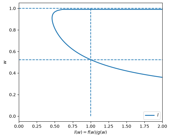
The two horizontal dashed lines mark the values of \(w\) at which \(l(w) = 1\).
Between them the likelihood ratio is below one, so by (28.3) a draw in that region pushes \(\pi\) down.
Outside them it exceeds one, so a draw there pushes \(\pi\) up.
28.7.2. The densities and the probabilities of moving in each direction#
Our second graph plots \(f(w)\) and \(g(w)\) against \(w\), and shades the regions delineated by those same two values of \(w\).
Shading them lets us attach a probability to each direction of movement, which we compute by integrating the relevant density over the region.
def plot_densities(F_a=1, F_b=1, G_a=3, G_b=1.2):
    f, g, roots = create_model(F_a, F_b, G_a, G_b)
    w_grid = np.linspace(0, 1, 100)

    fig, ax = plt.subplots(figsize=(6, 5))
    ax.plot(f(w_grid), w_grid, label='$f$', lw=2)
    ax.plot(g(w_grid), w_grid, label='$g$', lw=2)
    ax.vlines(1, 0, 1, linestyle='--')
    ax.hlines(roots, 0, 2, linestyle='--')
    ax.legend(loc=4)
    ax.set(xlabel='$f(w), g(w)$', ylabel='$w$')

    # Probability of landing in each region, under whichever density is shaded
    area_lower = quad(f, 0, roots[0])[0]
    area_middle = quad(g, roots[0], roots[1])[0]
    area_upper = quad(f, roots[1], 1)[0]

    ax.fill_between([0, 1], 0, roots[0], color='blue', alpha=0.15)
    ax.text((f(0) + f(roots[0])) / 4, roots[0] / 2, f"{area_lower: .3g}")
    w_middle = np.linspace(roots[0], roots[1], 20)
    ax.fill_betweenx(w_middle, 0, g(w_middle), color='orange', alpha=0.15)
    ax.text(np.mean(g(roots)) / 2, np.mean(roots), f"{area_middle: .3g}")
    ax.fill_between([0, 1], roots[1], 1, color='blue', alpha=0.15)
    ax.text((f(roots[1]) + f(1)) / 4, (roots[1] + 1) / 2, f"{area_upper: .3g}")
    plt.show()
Let’s look at the same pair of distributions as before.
plot_densities()
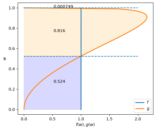
The fractions in the colored areas are probabilities that a realization of \(w\) falls into the region beside them.
The blue regions are integrals of \(f\) and the orange region is an integral of \(g\).
For example, under true distribution \(F\), \(\pi\) will be updated toward \(0\) if \(w\) falls into the interval \([0.524, 0.999]\), which occurs with probability \(1 - .524 = .476\) under \(F\).
But this would occur with probability \(0.816\) if \(G\) were the true distribution.
28.7.3. Dynamics of the belief#
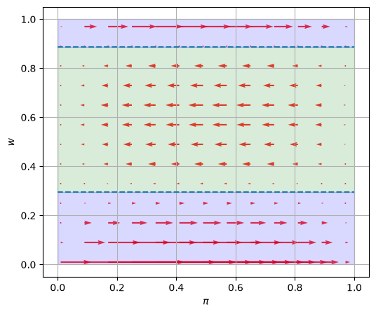
Our third graph attaches an arrow to each point in the \((\pi, w)\) plane showing the change in \(\pi\) that Bayes’ Law induces when the current belief is \(\pi\) and the new draw is \(w\).
def plot_belief_dynamics(F_a=1, F_b=1, G_a=3, G_b=1.2):
    f, g, roots = create_model(F_a, F_b, G_a, G_b)
    π_grid = np.linspace(1e-3, 1 - 1e-3, 100)

    # Change in π at each point of a coarse grid over (π, w)
    W = np.arange(0.01, 0.99, 0.08)
    Π = np.arange(0.01, 0.99, 0.08)
    lw = (f(W) / g(W))[:, None]     # likelihood ratio at each w, as a column
    ΔΠ = Π * (lw / (Π * lw + 1 - Π) - 1)
    ΔW = np.zeros_like(ΔΠ)

    fig, ax = plt.subplots(figsize=(6, 5))
    ax.quiver(Π, W, ΔΠ, ΔW, scale=2, color='r', alpha=0.8)
    ax.fill_between(π_grid, 0, roots[0], color='blue', alpha=0.15)
    ax.fill_between(π_grid, roots[0], roots[1], color='green', alpha=0.15)
    ax.fill_between(π_grid, roots[1], 1, color='blue', alpha=0.15)
    ax.hlines(roots, 0, 1, linestyle='--')
    ax.set(xlabel=r'$\pi$', ylabel='$w$')
    ax.grid()
    plt.show()
Again we use the same pair of distributions.
plot_belief_dynamics()
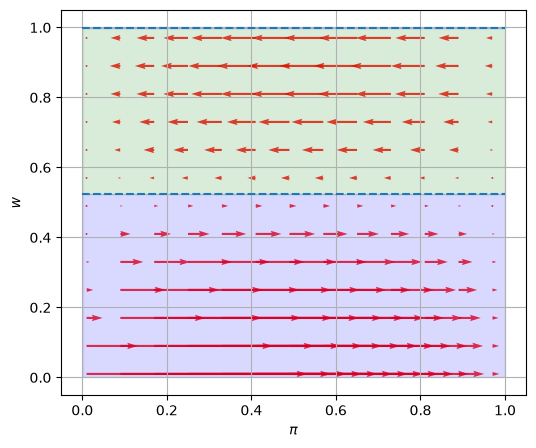
Arrows pointing right show when Bayes’ Law makes \(\pi\) increase and arrows pointing left show when it makes \(\pi\) decrease.
Lengths of the arrows show magnitudes of the force from Bayes’ Law impelling \(\pi\) to change.
These lengths depend on both the prior probability \(\pi\) on the abscissa axis and the evidence in the form of the current draw of \(w\) on the ordinate axis.
Arrows point right in the blue regions, where \(l(w) > 1\), and left in the green region between the dashed lines, where \(l(w) < 1\).
For these parameters the upper blue region is a thin sliver just below \(w = 1\), since \(l(w)\) returns above one only for draws very close to the upper limit.
28.7.4. Another instance#
Next we use our code to create graphs for another instance of our model.
We keep \(F\) the same as in the preceding instance, namely a uniform distribution, but now assume that \(G\) is a Beta distribution with parameters \(G_a=2, G_b=1.6\).
plot_likelihood_ratio(G_a=2, G_b=1.6)
plot_densities(G_a=2, G_b=1.6)
plot_belief_dynamics(G_a=2, G_b=1.6)
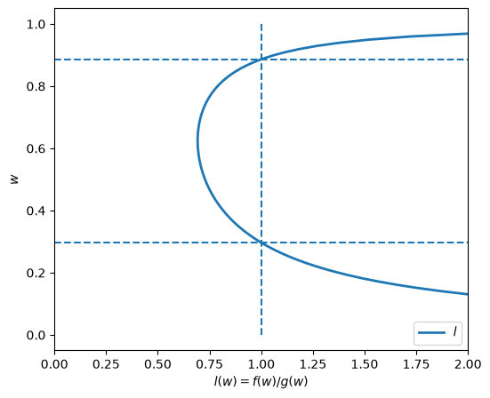
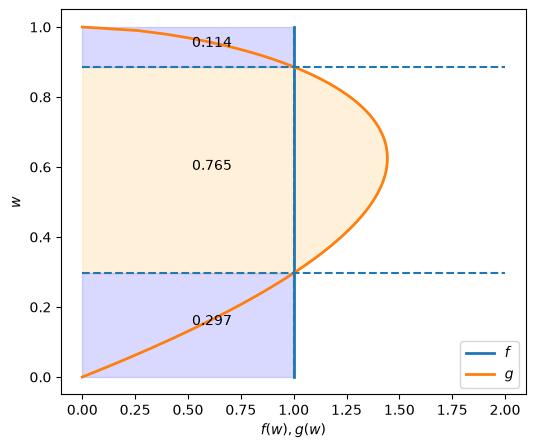
Notice how the likelihood ratio, the densities, and the arrows compare with the previous instance of our example.
28.8. Appendix#
28.8.1. Sample paths of \(\pi_t\)#
Now we’ll have some fun by plotting multiple realizations of sample paths of \(\pi_t\) under two possible assumptions about nature’s choice of distribution, namely
that nature permanently draws from \(F\)
that nature permanently draws from \(G\)
Outcomes depend on a peculiar property of likelihood ratio processes discussed in Additive and Multiplicative Functionals.
Before simulating, it pays to rewrite Bayes’ Law in terms of odds rather than probabilities.
In terms of the odds \(\pi / (1 - \pi)\), the updating rule (28.2) becomes
So Bayes’ Law is multiplicative in the odds, and iterating (28.4) back to the prior \(\pi_{-1}\) yields
The belief path is thus a running product of likelihood ratios, which is why properties of likelihood ratio processes govern its behavior.
It also means that we can simulate an entire ensemble of paths with a cumulative product, with no iteration over dates.
def simulate(rng, a, b, T=50, N=1000, π_init=0.5,
             F_a=1, F_b=1, G_a=3, G_b=1.2):
    """
    Simulate N paths of the belief π over T periods, when nature draws IID
    from Beta(a, b).  Returns an array of shape (N, T+1) whose first column
    holds the common prior π_init.
    """
    w = rng.beta(a, b, size=(N, T))
    l = p(w, F_a, F_b) / p(w, G_a, G_b)
    odds = (π_init / (1 - π_init)) * np.cumprod(l, axis=1)
    return np.column_stack([np.full(N, π_init), odds / (1 + odds)])
The paths are plotted by the next function.
def plot_paths(π_paths):
    fig, ax = plt.subplots()
    ax.plot(π_paths.T, color='b', lw=0.8, alpha=0.5)
    ax.set(xlabel='$t$', ylabel=r'$\pi_t$')
    plt.show()
We begin by generating \(N\) simulated \(\{\pi_t\}\) paths with \(T\) periods when the sequence is truly IID draws from \(F\). We set an initial prior \(\pi_{-1} = .5\).
rng = np.random.default_rng(42)
T = 50
# when nature selects F
π_paths_F = simulate(rng, a=1, b=1, T=T, N=1000)
plot_paths(π_paths_F)
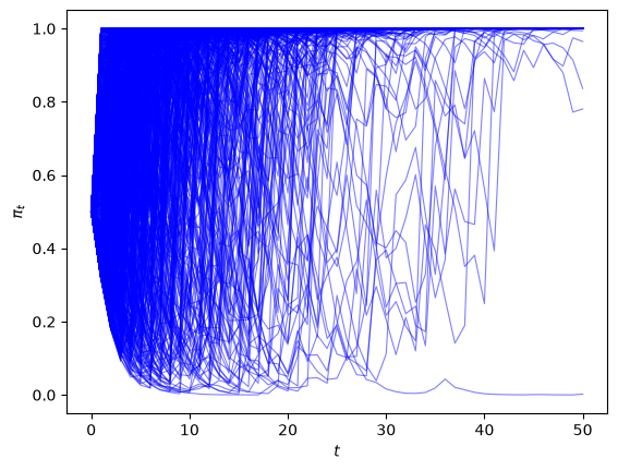
In the above example, for most paths \(\pi_t \rightarrow 1\).
So Bayes’ Law evidently eventually discovers the truth for most of our paths.
Next, we generate paths with \(T\) periods when the sequence is truly IID draws from \(G\). Again, we set the initial prior \(\pi_{-1} = .5\).
# when nature selects G
π_paths_G = simulate(rng, a=3, b=1.2, T=T, N=1000)
plot_paths(π_paths_G)
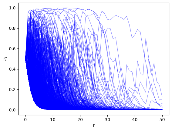
In the above graph we observe that now most paths \(\pi_t \rightarrow 0\).
28.8.2. Rates of convergence#
We study rates of convergence of \(\pi_t\) to \(1\) when nature generates the data as IID draws from \(F\) and of convergence of \(\pi_t\) to \(0\) when nature generates IID draws from \(G\).
We do this by averaging across simulated paths of \(\{\pi_t\}_{t=0}^T\).
Using \(N\) simulated \(\pi_t\) paths, we compute \(1 - \sum_{i=1}^{N}\pi_{i,t}\) at each \(t\) when the data are generated as draws from \(F\) and compute \(\sum_{i=1}^{N}\pi_{i,t}\) when the data are generated as draws from \(G\).
fig, ax = plt.subplots()
ax.plot(range(T + 1), 1 - np.mean(π_paths_F, axis=0), label='F generates')
ax.plot(range(T + 1), np.mean(π_paths_G, axis=0), label='G generates')
ax.set(xlabel='$t$', title='convergence')
ax.legend()
plt.show()
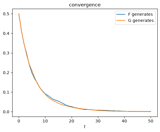
From the above graph, rates of convergence appear not to depend on whether \(F\) or \(G\) generates the data.
28.8.3. Graph of ensemble dynamics of \(\pi_t\)#
More insights about the dynamics of \(\{\pi_t\}\) can be gleaned by computing conditional expectations of \(\frac{\pi_{t+1}}{\pi_{t}}\) as functions of \(\pi_t\) via integration with respect to the pertinent probability distribution:
where \(a =f,g\).
The following code approximates the integral above:
def plot_expected_ratio(F_a=1, F_b=1, G_a=3, G_b=1.2):
    # Build f and g directly: here they can coincide, so l(w) = 1 has no root
    f = lambda w: p(w, F_a, F_b)
    g = lambda w: p(w, G_a, G_b)
    l = lambda w: f(w) / g(w)
    π_grid = np.linspace(0.02, 0.98, 100)

    fig, ax = plt.subplots()
    for label, a in [('f', f), ('g', g)]:
        integrand = lambda w, π: a(w) * l(w) / (π * l(w) + 1 - π)
        ratios = [quad(integrand, 0, 1, args=(π,))[0] for π in π_grid]
        ax.plot(π_grid, ratios, label=f'{label} generates')

    ax.hlines(1, 0, 1, linestyle='--')
    ax.set(xlabel=r'$\pi_t$', ylabel=r'$E[\pi_{t+1} / \pi_t]$')
    ax.legend()
    plt.show()
First, consider the case where \(F_a=F_b=1\) and \(G_a=3, G_b=1.2\).
plot_expected_ratio()
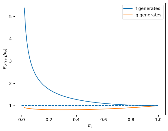
The above graph shows that when \(F\) generates the data, \(\pi_t\) on average always heads north, while when \(G\) generates the data, \(\pi_t\) heads south.
Next, we’ll look at a degenerate case in which \(f\) and \(g\) are identical beta distributions, and \(F_a=G_a=3, F_b=G_b=1.2\).
In a sense, here there is nothing to learn.
plot_expected_ratio(F_a=3, F_b=1.2)
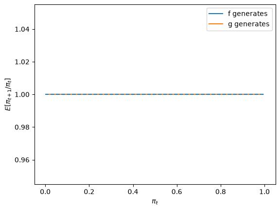
The above graph says that \(\pi_t\) is inert and remains at its initial value.
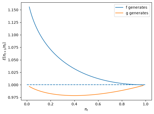
Finally, let’s look at a case in which \(f\) and \(g\) are neither very different nor identical, in particular one in which \(F_a=2, F_b=1\) and \(G_a=3, G_b=1.2\).
plot_expected_ratio(F_a=2, F_b=1, G_a=3, G_b=1.2)
28.9. Sequels#
We’ll apply and dig deeper into some of the ideas presented in this lecture:
Likelihood Ratio Processes describes likelihood ratio processes and their role in frequentist and Bayesian statistical theories
Bayesian versus Frequentist Decision Rules studies whether a World War II US Navy Captain’s hunch that a (frequentist) decision rule that the Navy had told him to use was inferior to a sequential rule that Abraham Wald had not yet designed.