25. Mean of a Likelihood Ratio Process#
GPU
This lecture was built using a machine with access to a GPU — although it will also run without one.
Google Colab has a free tier with GPUs that you can access as follows:
Click on the “play” icon top right
Select Colab
Set the runtime environment to include a GPU
25.1. Overview#
In Likelihood Ratio Processes we described a peculiar property of a likelihood ratio process, namely, that its mean equals one for all \(t \geq 0\) despite its converging to zero almost surely.
While it is easy to verify that peculiar property analytically (i.e., in population), it is challenging to use a computer simulation to verify it via an application of a law of large numbers that entails studying sample averages of repeated simulations.
To confront this challenge, this lecture puts importance sampling to work to accelerate convergence of sample averages to population means.
We use importance sampling to estimate the mean of a cumulative likelihood ratio \(L\left(\omega^t\right) = \prod_{i=1}^t \ell \left(\omega_i\right)\).
In addition to what’s in Anaconda, this lecture will need the following libraries:
!pip install jax
We start by importing some Python packages.
import jax
import jax.numpy as jnp
import numpy as np
import matplotlib.pyplot as plt
from jax.scipy.stats import beta
from typing import NamedTuple
from functools import partial

# Set JAX to use 64-bit floats
jax.config.update("jax_enable_x64", True)
25.2. Mathematical expectation of likelihood ratio#
In Likelihood Ratio Processes, we studied a likelihood ratio \(\ell \left(\omega_t\right)\)
where \(f\) and \(g\) are densities for Beta distributions with parameters \(F_a\), \(F_b\), \(G_a\), \(G_b\).
Assume that an i.i.d. random variable \(\omega_t \in \Omega\) is generated by \(g\).
The cumulative likelihood ratio \(L \left(\omega^t\right)\) is
Our goal is to approximate the mathematical expectation \(E \left[ L\left(\omega^t\right) \right]\) well.
In Likelihood Ratio Processes, we showed that \(E \left[ L\left(\omega^t\right) \right]\) equals \(1\) for all \(t\).
We want to check out how well this holds if we replace \(E\) with sample averages from simulations.
This turns out to be easier said than done because for Beta distributions assumed above, \(L\left(\omega^t\right)\) has a very skewed distribution with a very long tail as \(t \rightarrow \infty\).
This property makes it difficult efficiently and accurately to estimate the mean by standard Monte Carlo simulation methods.
In this lecture we explore how a standard Monte Carlo method fails.
We also show how importance sampling provides a more computationally efficient way to approximate the mean of the cumulative likelihood ratio.
We first take a look at the density functions f and g .
# Parameters for the model
class ImpSampleParams(NamedTuple):
    F_a: float = 1.0    # Beta parameters for f
    F_b: float = 1.0
    G_a: float = 3.0    # Beta parameters for g
    G_b: float = 1.2

params = ImpSampleParams()

def f(w):
    return beta.pdf(w, params.F_a, params.F_b)

def g(w):
    return beta.pdf(w, params.G_a, params.G_b)
w_range = np.linspace(1e-2, 1-1e-5, 1000)

plt.plot(w_range, g(w_range), lw=2, label='g')
plt.plot(w_range, f(w_range), lw=2, label='f')
plt.xlabel(r'$\omega$')
plt.legend()
plt.show()
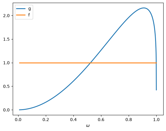
Fig. 25.1 Beta density functions \(f\) and \(g\)#
The likelihood ratio is l(w)=f(w)/g(w).
def l(w):
    return f(w) / g(w)
plt.plot(w_range, l(w_range), lw=2)
plt.yscale('log')
plt.xlabel(r'$\omega$')
plt.ylabel(r'$\ell(\omega)$')
plt.show()
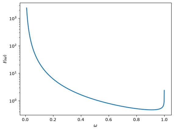
Fig. 25.2 Likelihood ratio \(\ell(\omega)\), log scale#
Note the log scale on the vertical axis: on a linear scale the entire curve would be flattened against zero by the spike at the left-hand edge.
Fig. 25.1 shows that as \(\omega \rightarrow 0\), \(f \left(\omega\right)\) is unchanged while \(g \left(\omega\right) \rightarrow 0\).
Hence the likelihood ratio in Fig. 25.2 diverges to infinity, at rate \(\omega^{-2}\).
The same thing happens as \(\omega \rightarrow 1\), since \(G_b > 1\) also forces \(g\left(\omega\right) \rightarrow 0\) there, which explains the upturn at the right-hand edge.
But that divergence is far slower — at rate \(\left(1-\omega\right)^{-1/5}\) — and it is the behavior near \(\omega = 0\) that causes the trouble below.
A Monte Carlo approximation of \(E \left[L\left(\omega^t\right)\right]\) would repeatedly draw a sequence \(\omega^t = \left(\omega_1, \ldots, \omega_t\right)\) of \(t\) independent observations from \(g\), form the product \(L\left(\omega^t\right) = \prod_{i=1}^t \ell \left(\omega_i\right)\) for each such sequence, then average these products across independently drawn sequences.
Because \(g(\omega) \rightarrow 0\) as \(\omega \rightarrow 0\), such a simulation procedure undersamples a part of the sample space \([0,1]\) that it is important to visit often in order to do a good job of approximating the mathematical expectation of \(\ell \left(\omega\right)\).
Every one of the \(t\) factors in \(L\left(\omega^t\right)\) is distorted in the same way, so the problem compounds as \(t\) grows.
We illustrate this numerically below.
25.3. Importance sampling#
We circumvent the issue by using a change of distribution called importance sampling.
Instead of drawing from \(g\) to generate data during the simulation, we use an alternative distribution \(h\) to generate draws of \(\omega\).
The idea is to design \(h\) so that it oversamples the region of \(\Omega\) where \(\ell \left(\omega_t\right)\) has large values but low density under \(g\).
After we construct a sample in this way, we must then weight each realization by the likelihood ratio of \(g\) and \(h\) when we compute the empirical mean of the likelihood ratio.
By doing this, we properly account for the fact that we are using \(h\) and not \(g\) to simulate data.
To illustrate, suppose we were interested in \({E}\left[\ell\left(\omega\right)\right]\).
We could simply compute:
where \(\omega_i^g\) indicates that \(\omega_i\) is drawn from \(g\).
But using our insight from importance sampling, we could instead calculate the object:
where \(\omega_i\) is now drawn from importance distribution \(h\).
Notice that the above two are exactly the same population objects:
25.4. Selecting a sampling distribution#
Since we must use an \(h\) that has larger mass in parts of the distribution to which \(g\) puts low mass, we use \(h=Beta(0.5, 0.5)\) as our importance distribution.
The plots compare \(g\) and \(h\).
g_a, g_b = params.G_a, params.G_b
h_a, h_b = 0.5, 0.5
w_range = np.linspace(1e-5, 1-1e-5, 1000)

plt.plot(w_range, g(w_range),
         lw=2, label=f'g=Beta({g_a}, {g_b})')
plt.plot(w_range, beta.pdf(w_range, 0.5, 0.5),
         lw=2, label=f'h=Beta({h_a}, {h_b})')
plt.legend()
plt.ylim([0., 3.])
plt.show()
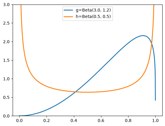
Fig. 25.3 Data and importance sampling distributions#
25.5. Approximating a cumulative likelihood ratio#
We now study how to use importance sampling to approximate \({E} \left[L\left(\omega^t\right)\right] = E \left[\prod_{i=1}^t \ell \left(\omega_i\right)\right]\).
As above, our plan is to draw sequences \(\omega^t\) from \(q\) and then re-weight the likelihood ratio appropriately.
The change of distribution holds in population, exactly as it did for a single draw:
This suggests the estimator
where \(\omega_{n,i}^q\) is the \(i\)-th observation of the \(n\)-th sequence, drawn from the importance distribution \(q\).
Here \(\frac{p\left(\omega_{n,i}^q\right)}{q\left(\omega_{n,i}^q\right)}\) is the weight we assign to each data point \(\omega_{n,i}^q\).
Below we prepare a Python function for computing the importance sampling estimates given any beta distributions \(p\), \(q\).
def estimate_single_path(key, p_a, p_b, q_a, q_b, T):
    """
    Estimation for a single sample path.
    """

    def loop_body(i, carry):
        L, weight, key_state = carry
        key_state, subkey = jax.random.split(key_state)
        w = jax.random.beta(subkey, q_a, q_b)

        # Keep draws off the boundary, where the log densities
        # below produce the undefined form 0 * inf
        w = jnp.clip(w, 1e-12, 1 - 1e-12)

        # Compute likelihood ratio using f/g functions
        likelihood_ratio = f(w) / g(w)
        L = L * likelihood_ratio

        # Importance sampling weight
        p_w = beta.pdf(w, p_a, p_b)
        q_w = beta.pdf(w, q_a, q_b)
        weight = weight * (p_w / q_w)

        return (L, weight, key_state)

    # Use fori_loop for dynamic T values
    final_L, final_weight, _ = jax.lax.fori_loop(
        0, T, loop_body, (1.0, 1.0, key)
    )
    return final_L * final_weight

@partial(jax.jit, static_argnames=['N'])
def estimate(key, p_a, p_b, q_a, q_b, T=1, N=10000):
    """Estimation of a batch of sample paths."""
    keys = jax.random.split(key, N)

    # Vectorize over keys, holding the parameters fixed
    estimates = jax.vmap(
        estimate_single_path,
        in_axes=(0, None, None, None, None, None)
    )(keys, p_a, p_b, q_a, q_b, T)

    return jnp.mean(estimates)
Consider the case when \(T=1\), which amounts to approximating \(E\left[\ell\left(\omega\right)\right]\).
For the standard Monte Carlo estimate, we can set \(p=g\) and \(q=g\).
estimate(jax.random.key(0), g_a, g_b, g_a, g_b,
         T=1, N=10000)
Array(0.98300826, dtype=float64)
For our importance sampling estimate, we set \(q = h\).
estimate(jax.random.key(1), g_a, g_b, h_a, h_b,
         T=1, N=10000)
Array(1.00722995, dtype=float64)
Evidently, even at \(T=1\), our importance sampling estimate is closer to \(1\) than is the Monte Carlo estimate.
Bigger differences arise when computing expectations over longer sequences, \(E\left[L\left(\omega^t\right)\right]\).
Setting \(T=10\), we find that the Monte Carlo method severely underestimates the mean while importance sampling still produces an estimate close to its theoretical value of unity.
estimate(jax.random.key(2), g_a, g_b, g_a, g_b,
         T=10, N=10000)
Array(0.60388316, dtype=float64)
estimate(jax.random.key(3), g_a, g_b, h_a, h_b,
         T=10, N=10000)
Array(0.99185478, dtype=float64)
The Monte Carlo method underestimates because the likelihood ratio \(L(\omega^T) = \prod_{t=1}^T \frac{f(\omega_t)}{g(\omega_t)}\) has a highly skewed distribution under \(g\).
Most samples from \(g\) produce small likelihood ratios, while the true mean requires occasional very large values that are rarely sampled.
In our case, since \(g(\omega) \to 0\) as \(\omega \to 0\) while \(f(\omega)\) remains constant, the Monte Carlo procedure undersamples precisely where the likelihood ratio \(\frac{f(\omega)}{g(\omega)}\) is largest.
In fact the situation is worse than skewness — the Monte Carlo estimator has infinite variance.
To see this, note that the second moment of a single likelihood ratio is
Here \(f\) is the uniform density, while \(g\left(\omega\right)\) vanishes like \(\omega^{G_a - 1} = \omega^2\) as \(\omega \to 0\).
The integrand therefore behaves like \(\omega^{-2}\) near the origin, and the integral diverges.
So \(\ell\left(\omega\right)\) has no finite variance, and since the draws are independent, neither does \(L\left(\omega^t\right)\) for any \(t\).
This is the precise sense in which standard Monte Carlo fails here: no central limit theorem applies to its sample averages, so they carry none of the usual \(\sqrt{N}\) guarantees.
As \(T\) increases, the problem worsens, making standard Monte Carlo increasingly unreliable.
Importance sampling with \(q = h\) fixes this by sampling more uniformly from regions important to both \(f\) and \(g\).
25.6. Distribution of sample mean#
We next study the bias and efficiency of the Monte Carlo and importance sampling approaches.
The code below repeats the estimate N_simu times, so that we can look at the distribution of the estimates that each method produces.
@partial(jax.jit, static_argnames=['N_simu', 'N_samples'])
def simulate(key, p_a, p_b, q_a, q_b, N_simu, T=1,
             N_samples=10000):
    """Repeat the estimate N_simu times, drawing from q."""
    keys = jax.random.split(key, N_simu)
    return jax.vmap(
        lambda k: estimate(k, p_a, p_b, q_a, q_b, T,
                           N_samples)
    )(keys)
Setting \(q = p\) recovers standard Monte Carlo, since every importance weight is then identically one.
Again, we first consider estimating \({E} \left[\ell\left(\omega\right)\right]\) by setting T=1.
We simulate \(1000\) times for each method.
N_simu = 1000
μ_L_g = simulate(jax.random.key(4), g_a, g_b,
                 g_a, g_b, N_simu)
μ_L_h = simulate(jax.random.key(5), g_a, g_b,
                 h_a, h_b, N_simu)
# standard Monte Carlo (mean and variance)
jnp.mean(μ_L_g), jnp.var(μ_L_g)
(Array(0.99558545, dtype=float64), Array(0.00448641, dtype=float64))
# importance sampling (mean and variance)
jnp.mean(μ_L_h), jnp.var(μ_L_h)
(Array(0.99985196, dtype=float64), Array(2.46227759e-05, dtype=float64))
Although both methods tend to provide a mean estimate of \({E} \left[\ell\left(\omega\right)\right]\) close to \(1\), the importance sampling estimates have smaller variance.
Next, we present distributions of estimates for \(\hat{E} \left[L\left(\omega^t\right)\right]\), in cases for \(T=1, 5, 10, 20\).
def simulate_multiple_T(key, p_a, p_b, q_a, q_b, T_values,
                        N_simu, N_samples=10000):
    """Run simulate once per T, returning a dict keyed by T."""
    keys = jax.random.split(key, len(T_values))
    return {T: simulate(keys[i], p_a, p_b, q_a, q_b,
                        N_simu, T, N_samples)
            for i, T in enumerate(T_values)}
The next function draws the histograms that we use to compare the two methods.
def plot_estimates(T_values, mc, imp, imp_label, n_rows=1):
    """Compare Monte Carlo and importance sampling estimates."""
    n_cols = len(T_values) // n_rows
    fig, axs = plt.subplots(n_rows, n_cols,
                            figsize=(14, 5 * n_rows))
    μ_range = np.linspace(0, 2, 100)

    for ax, T in zip(np.ravel(axs), T_values):
        μ_L_g, μ_L_h = np.asarray(mc[T]), np.asarray(imp[T])

        ax.set_xlabel('$μ_L$')
        ax.set_ylabel('frequency')
        ax.set_title(f'$T$={T}')
        ax.hist(μ_L_g, bins=μ_range,
                color='r', alpha=0.5, label='$g$ generating')
        ax.hist(μ_L_h, bins=μ_range,
                color='b', alpha=0.5, label=imp_label)
        ax.legend(loc=4)

        # Summarize each distribution in an upper corner
        for μ_L, color, x, ha in ((μ_L_g, 'r', 0.02, 'left'),
                                  (μ_L_h, 'b', 0.98, 'right')):
            ax.text(x, 0.98, transform=ax.transAxes, ha=ha,
                    va='top', color=color, fontsize=9,
                    s=r'$\hat{μ}$=' + f'{np.mean(μ_L):.3g}' +
                      '\n' + 'med=' + f'{np.median(μ_L):.3g}' +
                      '\n' + r'$\hat{σ}^2$=' + f'{np.var(μ_L):.3g}')

    plt.show()
The Monte Carlo estimates do not depend on the importance distribution, so we compute them once and reuse them in each of the figures below.
T_values = [1, 5, 10, 20]

mc = simulate_multiple_T(jax.random.key(6), g_a, g_b,
                         g_a, g_b, T_values, N_simu)
imp_h1 = simulate_multiple_T(jax.random.key(7), g_a, g_b,
                             h_a, h_b, T_values, N_simu)

plot_estimates(T_values, mc, imp_h1, '$h$ generating',
               n_rows=2)
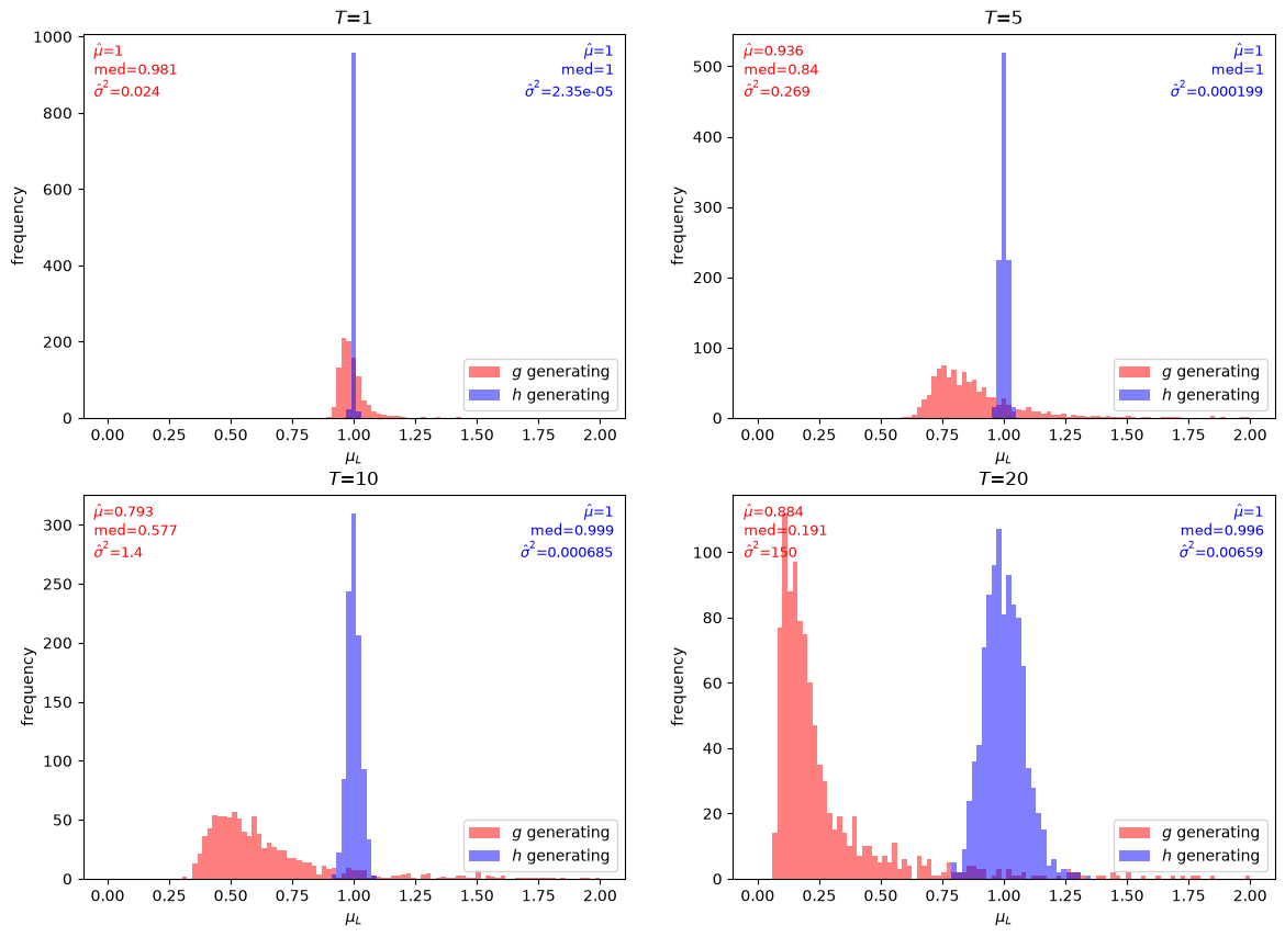
Fig. 25.4 Monte Carlo and importance sampling estimates#
The simulation exercises above show that the importance sampling estimates stay centered on \(1\) for every \(T\), while the distribution of the standard Monte Carlo estimates drifts steadily to the left as \(T\) increases.
It is worth being careful about what is going wrong here.
The Monte Carlo estimator is unbiased in population — its expectation is exactly \(1\) for every \(T\).
What deteriorates as \(T\) grows is the shape of its sampling distribution: almost all of the mass collapses towards zero, while the expectation is sustained by rare, very large outliers.
This is why each panel reports a median alongside the mean.
The median falls steadily in \(T\), whereas the reported mean \(\hat{μ}\) is an unreliable statistic — recall that the underlying variance is infinite, so the \(\hat{σ}^2\) printed in each panel estimates a quantity that does not exist, and a different seed can move \(\hat{μ}\) a long way.
Importance sampling repairs exactly this defect.
25.7. Choosing a sampling distribution#
Above, we arbitrarily chose \(h = Beta(0.5,0.5)\) as the importance distribution.
Is there an optimal importance distribution?
In our particular case, since we know in advance that \(E \left[ L\left(\omega^t\right) \right] = 1\), we can use that knowledge to our advantage.
Thus, suppose that we simply use \(h = f\).
When estimating the mean of the likelihood ratio (T=1), we get:
μ_L_f = simulate(jax.random.key(8), g_a, g_b,
                 params.F_a, params.F_b, N_simu)
# importance sampling (mean and variance)
jnp.mean(μ_L_f), jnp.var(μ_L_f)
(Array(1., dtype=float64), Array(6.40949485e-34, dtype=float64))
We could also use other distributions as our importance distribution.
Below we choose just a few and compare their sampling properties.
a_list = [0.5, 1., 2.]
b_list = [0.5, 1.2, 5.]
w_range = np.linspace(1e-5, 1-1e-5, 1000)

plt.plot(w_range, g(w_range),
         lw=2, label=f'g=Beta({g_a}, {g_b})')
plt.plot(w_range, beta.pdf(w_range, a_list[0], b_list[0]),
         lw=2, label=f'$h_1$=Beta({a_list[0]},{b_list[0]})')
plt.plot(w_range, beta.pdf(w_range, a_list[1], b_list[1]),
         lw=2, label=f'$h_2$=Beta({a_list[1]},{b_list[1]})')
plt.plot(w_range, beta.pdf(w_range, a_list[2], b_list[2]),
         lw=2, label=f'$h_3$=Beta({a_list[2]},{b_list[2]})')
plt.legend()
plt.ylim([0., 3.])
plt.show()
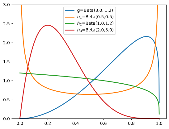
Fig. 25.5 Comparison of importance sampling distributions#
We consider two additional distributions.
As a reminder \(h_1\) is the original \(Beta(0.5,0.5)\) distribution that we used above.
\(h_2\) is the \(Beta(1,1.2)\) distribution.
Note how \(h_2\) has a similar shape to \(g\) at higher values of \(\omega\) but more mass at lower values.
Our hunch is that \(h_2\) should be a good importance sampling distribution.
\(h_3\) is the \(Beta(2,5)\) distribution.
Note how \(h_3\) has almost no mass at values very close to 0 and at values close to 1.
Our hunch is that \(h_3\) will be a poor importance sampling distribution.
The variance calculation above lets us make these hunches precise.
Drawing from \(h\) and reweighting gives each observation the value \(\ell\left(\omega\right) g\left(\omega\right) / h\left(\omega\right) = f\left(\omega\right) / h\left(\omega\right)\), so the estimator has finite variance exactly when
For \(h_1\) and \(h_2\) this integral converges.
For \(h_3\) it diverges at both endpoints, since \(h_3\) vanishes like \(\omega\) at the origin and like \(\left(1-\omega\right)^4\) at one.
So importance sampling with \(h_3\) has infinite variance, just as standard Monte Carlo does — which is what makes it a poor choice.
We first simulate and plot the distribution of estimates for \(\hat{E} \left[L\left(\omega^t\right)\right]\) using \(h_2\) as the importance sampling distribution.
T_values_h2 = [1, 20]
imp_h2 = simulate_multiple_T(jax.random.key(9), g_a, g_b,
                             a_list[1], b_list[1],
                             T_values_h2, N_simu)

plot_estimates(T_values_h2, mc, imp_h2, '$h_2$ generating')
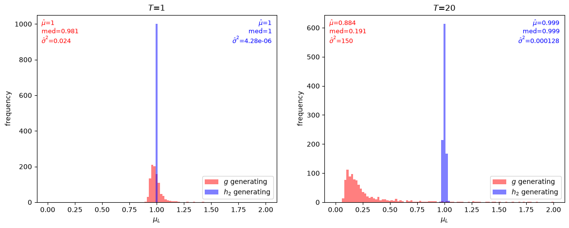
Fig. 25.6 Estimates using importance distribution \(h_2\)#
Our simulations suggest that indeed \(h_2\) is a quite good importance sampling distribution for our problem.
Even at \(T=20\), the mean is very close to \(1\) and the variance is small.
T_values_h3 = [1, 20]
imp_h3 = simulate_multiple_T(jax.random.key(10), g_a, g_b,
                             a_list[2], b_list[2],
                             T_values_h3, N_simu)

plot_estimates(T_values_h3, mc, imp_h3, '$h_3$ generating')
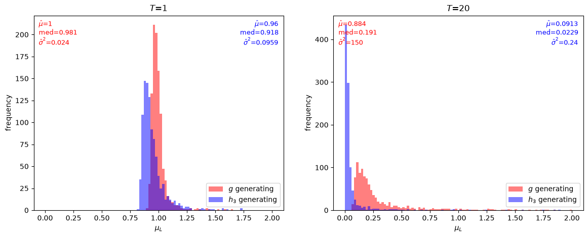
Fig. 25.7 Estimates using importance distribution \(h_3\)#
However, \(h_3\) is evidently a poor importance sampling distribution for our problem, with a mean estimate far away from \(1\) for \(T = 20\).
Notice that even at \(T = 1\), the mean estimate with importance sampling is more biased than sampling with just \(g\) itself.
Thus, our simulations suggest that for our problem we would be better off simply using Monte Carlo approximations under \(g\) than using \(h_3\) as an importance sampling distribution.